
When working on financial transactions, it’s easy to miss important details, especially during busy times like the end of the month or year.
The rush to meet deadlines can lead to wrong numbers or typing errors.
It’s important to format your Excel spreadsheet correctly to avoid these mistakes.
This means using bold titles, color-coding sections, and other simple tricks to organize your data, making it easier to spot and fix errors. This will help you create accurate financial reports.
10 Ways to Format Your Excel Spreadsheet
Excel is a powerful tool; properly formatting your spreadsheets can make them much easier to read and understand. These 10 tips will guide you in organizing your data effectively.
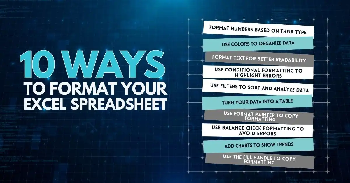
1. Format Numbers Based on Their Type (Like Money Values)
Formatting numbers in Excel help you make them look clear and easy to understand. For example, you can:
- Add currency symbols like $ to money amounts
- Show money with two decimal places to include cents
- Use commas to separate thousands, millions, or billions
How to Apply Number Formatting in Excel
- Select the cells you want to format by clicking and dragging your mouse over them, or click the first cell, hold Shift (Windows) or Command (Mac), and click the other cells.
- Go to the ‘Home’ tab in Excel and find the dropdown that says ‘General.’
- Click the dropdown and pick a number format like ‘Accounting’ to line up symbols and decimal points neatly in a column, making it easier to read the numbers.
- You can also right-click the selected cells, then click ‘Number Format,’ and from there, choose from more detailed options.
A box will pop up where you can select ‘Accounting’ and customize the settings. By default, there are two decimal places and a dollar sign ($). To change the currency symbol or remove decimal points, use the dropdown arrows.
Once you’re satisfied with the settings, simply click ‘OK’ to apply the formatting.
Other Useful Formatting Options
- Number – Use for general numbers; you can choose the number of decimal places, add commas for thousands, and show negative numbers in different ways.
- Currency – Great for money values; includes currency symbols, decimals, and commas.
- Short Date – Shows day, month, and year (like “4/13/2024”).
- Long Date – Adds the day of the week and full month name (like “Tuesday, April 13, 2024”).
- Time –Format time (like “1:45 PM” as “13:45:00”).
- Comma – Adds commas to large numbers (like “1,000”).
- Percentage – Converts numbers to percentages (like “50%” for 0.5).
- Fraction – Shows numbers as fractions (like “1/2” for 0.5).
- Special – Useful for things like ZIP codes or phone numbers.
- Custom – Lets you create your number formats.
2. Use Colors to Organize Data
Color-coding text in Excel helps you easily identify and understand different types of data. For instance, when reviewing sales data, you can use different colors to highlight how each product is performing.
- Review your data and decide what categories you want to color-code.
- Select the cells by clicking and dragging your mouse, or click the first cell, hold down Shift (Windows) or Command (Mac), and select the other cells.
- Go to the “Home” tab, click the dropdown next to the Fill Color icon, and choose your color.
Best Practices for Color-Coding
- Use green for positive numbers or gains.
- Use red for negative numbers or losses.
- Use neutral colors like gray for values that don’t need emphasis.
- Use bright colors to highlight important information.
- Use shades of the same color to show changes over time.
- Use dark text on light backgrounds for better readability.
3. Format Text for Better Readability
Well-formatted text makes your data easier to understand. Using bold, italics, and underlining can highlight key information, helping you navigate large datasets.
- Bold and Italics – To bold text, select the cells, go to the “Home” tab, and click the “B” icon. For italics, click the “I” icon.
- Font and Size – From the “Home” tab, choose the desired font and font size using the dropdown menus.
- Change Text Color – Click the dropdown next to the Font Color icon to pick a color for your text.
4. Use Conditional Formatting to Highlight Errors
Conditional formatting automatically changes the appearance of cells based on their values. For example, you can simplify and highlight any value over $1,000 in red.
- Select the cells you want to apply the rule to.
- In the “Home” tab, click “Conditional Formatting.”
- First, choose “Highlight Cell Rules” and then select “Greater Than.” Next, enter the desired value (e.g., 1000) and choose a color to highlight these values.
5. Use Filters to Sort and Analyze Data
Filters make it easy to sort or filter your data based on categories, dates, or amounts.
- Select the cells you want to filter, go to the “Data” tab, and click “Filter.”
- Click the dropdown arrows next to each column header and choose how you want to sort or filter the data.
6. Turn Your Data into a Table
Turning data into a table makes it easier to read and sort. It also allows you to use AI-powered tools like Microsoft Copilot.
- Select the cells containing your data.
- In the “Home” tab, click “Format as Table” and pick a style.
7. Use Format Painter to Copy Formatting
Format Painter helps you quickly copy one cell’s formatting to other cells.
- Select the cell from which you want to copy the format.
- First, click the “Format Painter” icon in the “Home” tab. Next, select the cells you want to apply the format to.
8. Use Balance Check Formatting to Avoid Errors
Balance Check Formatting helps you catch mistakes in your spreadsheets. It lets you compare the total of all items to ensure nothing is missing.
- Create a formula below your total that adds all individual items.
- Subtract the total from this sum—something is missing if the result isn’t zero.
9. Add Charts to Show Trends
Charts help visualize data trends and patterns.
- Select the data you want to visualize.
- Go to the “Insert” tab, choose “Charts,” and pick the chart type that best fits your data.
10. Use the Fill Handle to Copy Formatting
The Fill Handle is a small square at the corner of a selected cell. You can use it to copy formats to adjacent cells.
- First, select the formatted cell, then drag the Fill Handle over the cells you want to apply the format to.
- Click the “Auto Fill Options” icon and choose “Fill Formatting Only” to copy just the format.
Basic Excel Formulas for Everyday Transactions
In Excel, formulas allow you to perform math on groups of cells, providing instant results, even when there’s an error in your data. Additionally, they can be used to add, subtract, multiply, and divide, as well as calculate averages, and percentages, and work with dates and times.
Moreover, Excel offers a variety of formulas for different tasks. However, let’s focus on a few basic ones for everyday math and data operations.
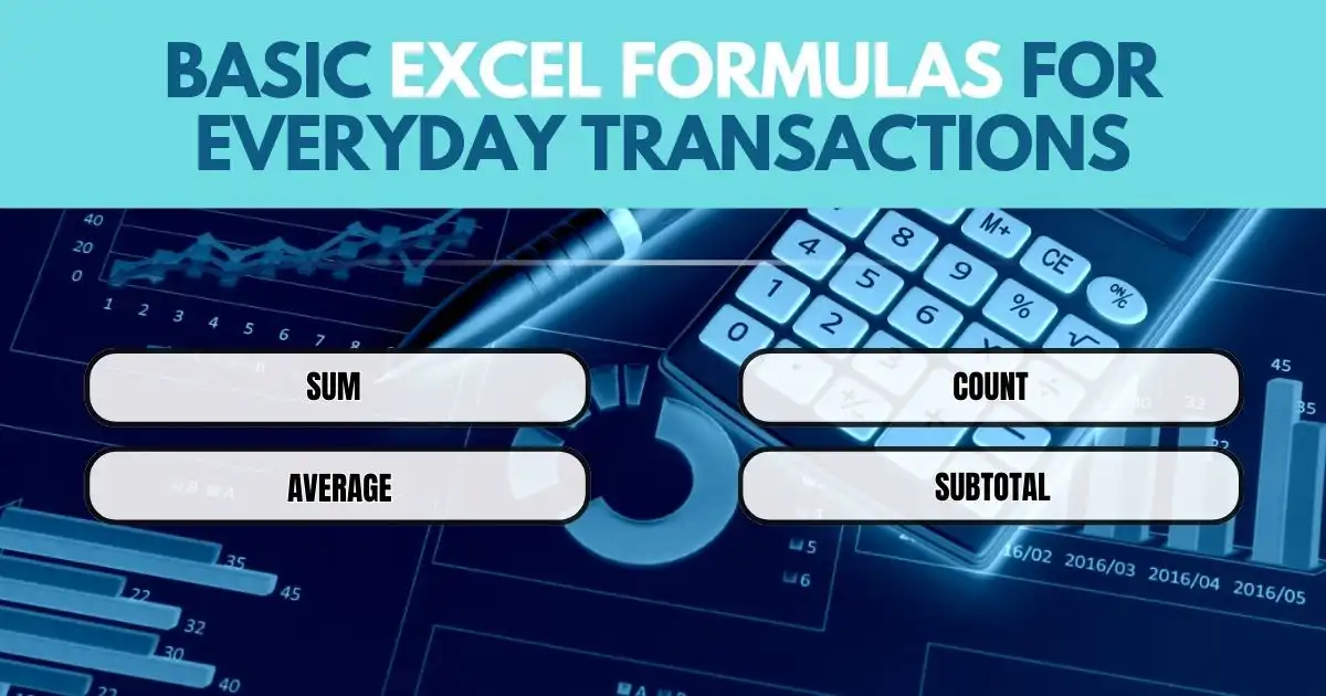
- Sum – The SUM() function adds up values in a selected range of cells. For instance, to calculate total sales, you can apply the formula =SUM(D7). This will add the numbers in cells D7 and D8, and as a result, the total will appear in cell D9.
- Average – The AVERAGE() function calculates the average of a group of cells. To find the average of total sales, just enter =AVERAGE(E5, E6, E7, E8, E9), and the average will be displayed in the cell you select.
- Count – The COUNT() function counts the number of cells in a range that contain numbers. For instance, using =COUNT(E5) will count the numerical values in the range E5 to E9 while ignoring any text or empty cells.
To count all cells with any data, including text, use the COUNTA() function. To count only blank cells, use COUNTBLANK().
- Subtotal – The SUBTOTAL() function allows you to perform operations like sum, count, or average on a specific range. For example, =SUBTOTAL(1, C5:C9) will calculate the average of the values in cells C5 to C9, while =SUBTOTAL(4, E5:E9) will find the maximum value in the selected range.
The Key to Error-Free Reports
When managing financial data, a well-formatted Excel spreadsheet can be the difference between clarity and chaos. Therefore, organizing your data properly is essential for ensuring smooth and accurate financial analysis. By using tools like bold headings, color-coding, and conditional formatting, you can make your data easier to read and minimize errors.
But here’s something to think about—are you taking full advantage of these features?
The next time you’re preparing an important report, try experimenting with different formatting techniques to see how much cleaner and more accurate your spreadsheet becomes. The right format could be the secret to not only catching mistakes but also presenting your data with confidence.
FAQs
Why are parts of my spreadsheet not working?
Parts of your spreadsheet might not work due to incorrect formulas, hidden columns, or formatting issues. Therefore, check for formula errors, ensure all cells are visible, and make sure the formatting is consistent.
What’s the best way to prepare reports in Excel?
Organize your data, use formulas for calculations, and add charts or graphs for visuals. Also, use headers, tables, and “Freeze Panes” to make reports clear and easily navigate.
What is the best font for Excel spreadsheets?
Arial, Calibri, and Verdana are the best fonts for readability and professional use. Therefore, they are simple, clear, and compatible across devices.
How do I copy the format from one Excel chart to another?
First, right-click the chart you want to copy. Next, select “Copy.” Then, right-click the target chart, choose “Paste Special,” and finally select “Formats” to apply the same design.